Problem definition

This verification problem considers production of a gasous component (zero-order production rate), equilibrium between the aqueous and liquid phase, and diffusion of a gaseous component to the atmosphere with a constant partial pressure of the gas component at the surface. There is no water flow.

Acronym 1DGAS02

Geometry

The profile has a length of 100 cm and consists of a single material.

Processes and Equations

The gas production rate is described by a first-order production term as:

where        C         is aqueous concentration

       t         is time

       γw         is the zero-order rate constant for the liquid phase [M/L³/T]

Initial and boundary conditions

The initial and boundary conditions are illustrated in Figure 1.

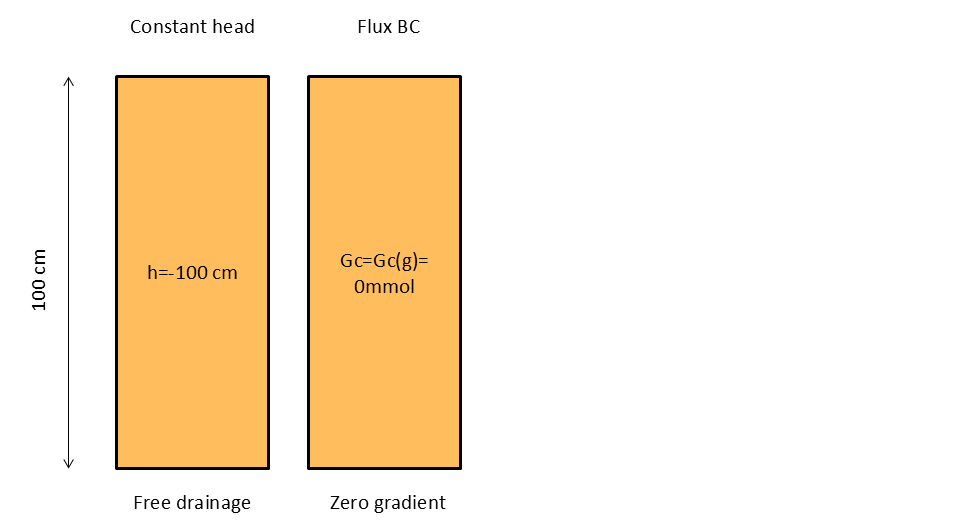
Figure 1 - Schematic representation of initial and boundary conditions for water flow (left) and solute transport (right)

The upper boundary constant head value is -100 cm.

The concentration in the atmosphere is 2.217 mol/m3 or a partial pressure of 5.424 10-2. A stagnant boundary layer of 0.01 m is assumed.

Material and Reaction Parameters

The hydraulic properties are described with the van Genuchten - Mualem model with m=1-1/n. Parameter values are in Table 1.

Table 1 - Parameters of the moisture retention curve and the unsaturated hydraulic conductivity as described with the model of van Genuchten -Mualem

The parameters of the solute transport equation and dispersion are given in Table 2.

Table 2 - Parameters of the solute transport equation (advection-dispersion equation with gas equilibrium).

The equilibrium constant between the gaseous and aqueous field as defined in HYDRUS-1D (kg) should be transformed to the thermodynamic constant for HPx (see Equivalence between parameter in HP and HYDRUS). The value is 10-1.462398.

The value for the zero-order rate constant for the liquid phase is 0.1 mol/m³/day.

Evaluation method

HPx simulations are compared with the calculations results of HYDRUS-1D. The output variables are:

• Time series of aqueous concentrations of the component Gc at depths of 5, 10, 20, 40, 75 and 100 cm, and
• Cumulative influx of gaseous Gc at the surface

Numerical Settings

The profile is discretized in 100 elements with 101 equally-spaced nodes.

The minimum and maximum time steps are 10-7 and 0.01 days, respectively.

The Crank-Nicholson scheme for time weighting and the Galarkin finite element scheme for space weighting are used with a stability criterion (PeCr) equal to 0.1.

Results

Figure 2 shows an excellent agreement between the time series of aqueous concentration of Gc obtained with HYDRUS-1D and HPx at selected depths.

Figure 3 shows an excellent agreement between the cumulative influx of gaseous Gc at the surface obtained with HYDRUS-1D and HPx.

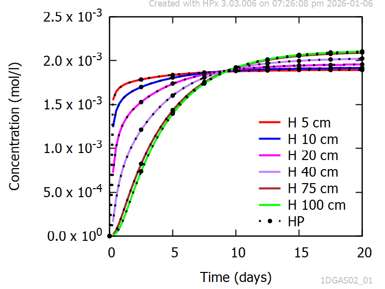
Figure 2 - Time series of aqueous concentrations of Gc for diffusive transport via the gas phase without any water transport (initial Gc free profile, constant partial pressure of Gc at the top boundary, zero-order production rate). Comparison between HPx and HYDRUS-1D.

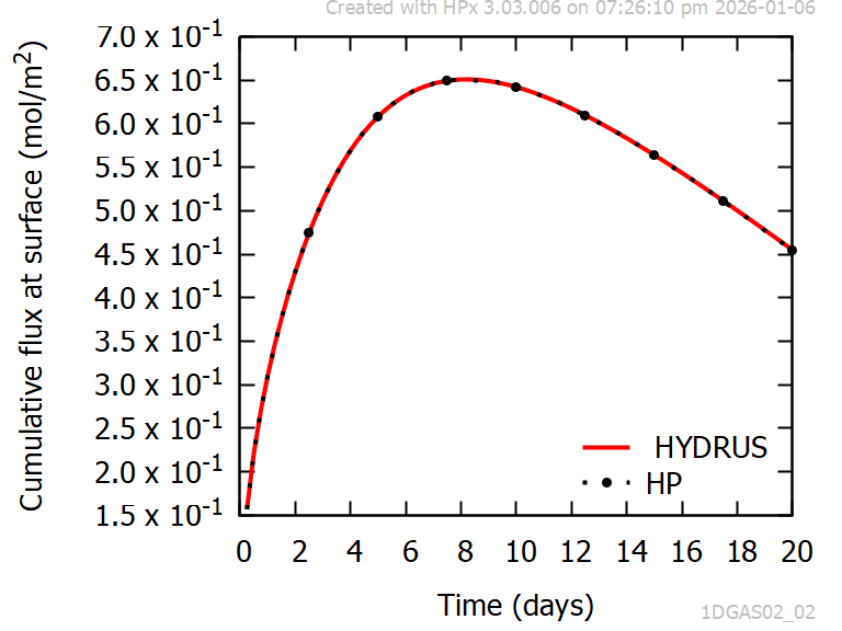
Figure 3 - Time series of cumulative influx of Gc at the top boundary for diffusive transport via the gas phase without any water transport (initial Gc free profile, constant partial pressure of Gc at the top boundary, zero-order production rate). Comparison between HPx and HYDRUS-1D.

Project HYDRUS 5.x

HPx - 1DGAS02-HPx.hyd5