1D - Tracer pulse during steady-state flow conditions

Problem Definition

This example describes the transport of a tracer under steady-state flow conditions in a one-dimensional profile. The aim is to verify the coupling of HYDRUS-1D and a given geochemical solver.

Acronym: ADR-T-SS

Geometry

The profile has a length of 100 cm and consists of a single material.

Processes and Equations

Water flow equation	Richards' equation	vertical flow (α=1), no water sink (S=0)
Solute transport	Advection-dispersion equation

Initial and boundary conditions

The initial and boundary conditions are illustrated in Figure 1.

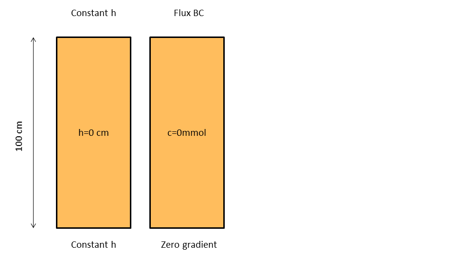
Figure 1 - Schematic representation of initial and boundary conditions for water flow (left) and solute transport (right)

The upper boundary condition for mass transport is a time-variable flux boundary condition with

c0 = 0.1 mol/kgw for 0 ≤ t ≤ 50d

c0 = 0.0 mol/kgw for 50 ≤ t ≤ 300d

Material Parameters

The hydraulic properties are described with the van Genuchten - Mualem model with m=1-1/n. Parameter values are in Table 1.

Table 1 - Parameters of the moisture retention curve and the unsaturated hydraulic conductivity as described with the model of van Genuchten -Mualem.

θs	0.43
θr	0.078
α	0.036 /cm
n	1.56
Ks	24.96 cm/days
l	0.5

The parameters of the solute transport equation and dispersion are given in Table 2.

Table 2 - Parameters of the solute transport equation (advection-dispersion equation)

DL	8 cm
Dw	0 cm2/day
τ	Millington & Quirk

Evaluation method

HPx simulations are compared with the calculations results of HYDRUS-1D. The output variables are:

Time series of concentrations at depths of 3, 25, 50, 75 and 100 cm, and
Concentration profiles at times 10, 20, 50, 100, 200 and 300 days.

Numerical Settings

The profile is discretized in 100 elements with 101 equally-spaced nodes.

The minimum and maximum time steps are 10-5 and 5 days, respectively (the latter being limited by the 0.5 day time step of output).

The Crank-Nicholson scheme for time weighting and the Galarkin finite element scheme for space weighting are used with a stability criterion (PeCr) equal to 2.

Results

Figure 2 shows an excellent agreement between the tracer breakthrough curves obtained with HP1 and HYDRUS-1D for the evolution to the tracer concentration at selected depths.

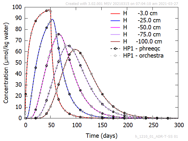
Figure 2 - Time series of tracer concentrations at selected depths during pulse application under steady-state flow conditions. Comparison between HPx and HYDRUS-1D.

Figure 3 shows an excellent agreement of tracer profiles at selected times obtained with HP1 and HYDRUS-1D.

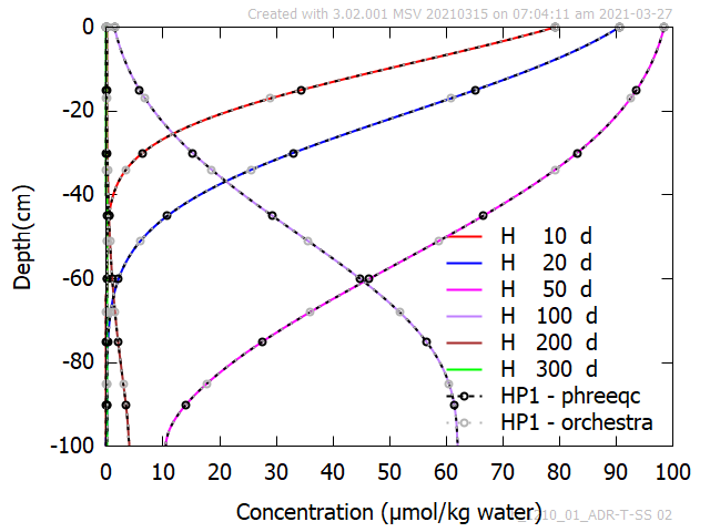
Figure 3 - Profiles of tracer concentrations at selected times during pulse application under steady-state flow conditions. Comparison between HPx and HYDRUS-1D.